Lab 5: Answering A Spatial Question of Our Own

     For Lab 5 our goal was to come up with our own spatial question to answer using the GIS tools and skills that we have developed over the course. The only restrictions we were given was that we needed to answer a simple yet relevant question using at least three different tools and have a total of four or more tool processes while answering our question. We were to choose a county anywhere in the U.S. to focus our question and use existing data provided from a variety of resources.

     My Major at UW - Eau Claire is in Ecology and Environmental Biology, so I wanted to ask a question that was relevant to Biology in Wisconsin. While thinking of the Wisconsin Department of Natural Resources I remembered work in previous courses about the Wisconsin wolf population. The population of wolves has changed in this state in recent years with the population tripling between 2000 and 2012. This and other factors led to the beginning of a hunting and trapping season for wolves in 2012.

     With these changes came rising popular interest in Wisconsin's wolves and the wolf population. The DNR drafted and implemented its own survey of Attitudes Towards Wolves and Wolf Management earlier this year, 2014. The results are interesting in their own right, but what I noticed was that the survey listed Eau Claire County as an outlier in its data. This was because the territory for wolves in Eau Claire County is concentrated in the far Eastern side of the county, while the greater population of people resides on the west side of the county. The survey was done by clustering counties into groups based on the percent of wolf territory and human population density in each county. It was hypothesized that Eau Claire county would be an outlier because in a smaller cluster it represents a large number of addresses with few of those addresses actually in wolf territories.

     Surveys were sent out to addresses randomly pulled from each group of clusters to be returned to the DNR. Unfortunately, the surveys only had a 59% return rate. Of those that were returned, 15% were also not fully completed upon return, usually due to people opting out of the survey for various reasons. This meant that of the 8,750 surveys that were sent out, only about 4,400 were returned completed; a total of only 50%. Poor return rates like this could skew data if some county clusters are more heavily represented than others.

     My question is, could we use data about habitat types, cities, and addresses to develop a survey for Eau Claire County?

     My main goal for this project was to make the table(s) of addresses, the residents of which would be asked to participate in an Eau Claire County wolf attitude survey.

     To increase data quality and accuracy, as well as increase the likelihood of getting the proper number of surveys from all representative areas, the survey of Eau Claire County should be administered orally. This wold not only allow for consistency in data entry, but it would allow the person administering the questionnaire to answer any questions about, or aide in understanding of the questionnaire. For this reason, addresses will be chosen within one kilometer of either side of highways, allowing enough distance from roads for proper habitat, while also keeping the surveyor on main roadways to streamline and better control time.

     Another issue with the DNR survey is that the addresses were chosen randomly across entire counties or clusters of counties. It does not compensate for the larger quantity of addresses that reside within cities. Wisconsin has a population of 5.74 million people, but only 1.5 million live in rural areas according to the USDA Economic Research Service. Wolves are more likely to be seen in a rural environment, so this survey will separate the addresses into urban and rural areas by defining urban areas as areas five kilometers from a city center.

     The survey will also separate the addresses based on the suitability of the local habitat for wolves. This will be used as a gauge for how likely a survey participant is to see a wolf, similar to the reason for distinguishing urban and rural areas. The Wisconsin DNR website provides a table of ecological landscapes and their level of association with wolves. This scales suitability for wolves from one to three in Eau Claire County, and these three categories along with the urban/rural distinction will make up the tables.

Objective I
     The first step to achieve these goals was to create a data flow model of each tool used and each feature obtained or created. I chose to do this in the program Visio rather than using ModelBuider in AcMap, because it can be used in free form and is more streamlined. (Results: Fig. 1)

Objective II
     The next thing that needed to be done was extracting data. Fortunately for me all of the necessary data and features were included on a university server. Otherwise it all would have been accessed by searching online and requesting data. Features were taken from the university server and placed in a new file geodatabase. This gives us a copy of the data in case it changes or is removed from the school server. It also keeps all the data in one place so it wont be difficult to seek out later. (Fig. 2)

Figure 2. contents of new file geodatabase
created for this project.

     All of the data was accessed from the university, however that data originally cam from sources like The Wisconsin DNR, ESRI GIS database, and information collected for the city of Eau Claire.

Objective III
     The data frame was then given a new coordinate system that would be appropriate for Eau Claire County. I chose the Central Wisconsin State Plane coordinate system because it can appropriately project the shape of the county.

Figure 3. All original features added and clipped to Eau Claire County Feature

     A feature of Eau Claire County was taken from a larger feature including all US counties and added to the database. This was added into ArcMap along with features of US highways, ecological landscapes, cities, and addresses. Each of these features were then individually projected to suit the state plane coordinate system using the projection tool in ArcMap. Each of these features were then reduced so that they fit within the boundaries of Eau Claire County. This was done using the clipping tool for each feature, with EC County used as the feature that all others were clipped by. (Fig. 3)

Objective IV
     Next we want to include the association with wolves to each ecological landscape. To do this I simply added a field to the ecological landscape attribute table and then, with editor running, I took the landscape score from the DNR website mentioned before and added it to the corresponding landscape. Doing this allows us to show the likelihood of a wolf sighting in each area.
    Now to distinguish urban areas it was necessary to add a buffer from each city center. This could be done using the buffer tool. I simply added a five kilometer buffer from the center of all cities, which does not account for the size of cities, however the largest city, Eau Claire, that best illustrates this problem has two small cities just outside it. When the buffer of the three cities combine it will act as a more appropriate approximation of the urban areas.
     I also used the buffer tool to create a feature showing an area one kilometer around highways that wold be used to find addresses for the survey. this was done in the same way as cities using the buffer tool.

Figure 4. Buffered City and Highway features.

     Adding a buffer caused the features to expand, pushing them beyond the boundaries of Eau Claire county. The buffered features had to clipped once again the same way the the non-buffered features were before. It would seem more logical to do this only once by first adding buffers to the original features and then clipping them to be within Eau Claire County. The original features covered the entirety of the United States, so it would have taken a long time to process both buffers and then clip them. (Fig. 4)

Objective V
     The next step was to begin dividing addresses that would be surveyed. They were divided by the ecological landscape or sighting likelihood as well as by urban or rural areas. This meant there would be six different features total. These would also be selected by their proximity to highways, so the addresses would be from six different areas, but all within one kilometer of a highway.
     I needed to first use the intersect tool to find the correct urban areas for addresses. In order to use only one part of the landscapes feature at a time (as opposed to breaking it into 3 features right away),
I needed to select one of the three landscapes using select by
attributes and then use the intersect tool. (Fig. 5). By intersecting the landscapes, buffered highways, and buffered cities features after this selection was made
(Fig. 6), I got single a feature of the area where all three previous features overlapped (Fig.7). This will be one of the six areas that needs to be created for selecting addresses. To better understand, here is a brief list of the selection and features intersected in urban areas:
Landscape 1 selection, buffered highways, buffered cities
Landscape 2 selection, buffered highways, buffered cities
Landscape 3 selection, buffered highways, buffered cities

Figure 6. Selecting the proper features to intersect.
The tool does not indicate that it is only using the
selected area of the landscapes feature. Simply
use the feature name and as long as only the desired
selection is made it will work properly.

Figure 5. Landscapes feature selection.

Figure 7. Product of intersect
tool function.

     The other half of the features needed would come from outside the urban areas. This required the erase tool. To do this I would select one of the three landscapes as before, and intersect it with only the buffered highways feature, giving the entire area within a landscape that might be surveyed (Fig. 8). Then I removed the urban areas from that feature using the erase tool (Fig 9). Here is another short list of the involved processes:
Intersect: Landscape 1 selection, buffered highways   Erase: buffered cities
Intersect: Landscape 2 selection, buffered highways   Erase: buffered cities
Intersect: Landscape 3 selection, buffered highways   Erase: buffered cities

Figure 8. Selection of greater survey
feature before use of the erasing tool.

Figure 9. Survey feature after
city feature is erased

     After this I had all six of the different survey areas needed to continue:
Urban areas of high landscape suitability for wolves near highways
Rural areas of high landscape suitability for wolves near highways
Urban areas of moderate landscape suitability for wolves near highways
Rural areas of moderate landscape suitability for wolves near highways
Urban areas of poor landscape suitability for wolves near highways
Rural areas of poor landscape suitability for wolves near highways
(Results: Fig. 10)

Objective VI
     Now that the six survey areas were determined, it was time to sort addresses by those that were within the survey features and between each of those different survey features. This simply required another intersection between each of the six survey feature and the address feature.

Objective VII
     The final step is to make all of the features shown cartographically pleasing. While the data tables themselves are too large to show, the features represented by them are displayed. Coloring each set of features to properly contrast the background is important in a situation like this where there is so much data. Adding a North arrow, scale bar, and legend is essential, but adding a visual reference of were the county is in Wisconsin was also needed. All address features were added, but the highway boundary from which they were chosen was added and had the color matched to each address feature to aide in the visualization of where those addresses were.(Results: Fig. 11)
    
Discussion
      Many ecologists would quickly point out a great shortcoming in the process of these surveys. It is pretty well documented that highways, much like cities, act as a habitat boundary to many animals. If this acts as a boundary for the wolves, then It would be a bad idea to only choose addresses within one kilometer on either side of the highway.
     This is a factor that would again limit the power of this survey. The problem is that this was also something that was already limited in the fact that most houses in Eau Claire county are within one kilometer of a highway (selecting addresses within the buffered highways feature shows 34,351 out of 39,172 addresses or nearly 88% are within one km). This may be something entirely unavoidable, with solutions not practically applicable in this type of survey.
     I spoke earlier about choosing certain numbers of people proportionally. There are a number of ways this could be done. One way would be to simply take an even number of people from each of the six categories. Another may be to determine the total area of each category and determine the number of addresses per square mile. Then one could tae te nuber of addresses per square mile and normalize it, giving fewer surveys in areas of higher density s that the number of surveys taken per square mile is more even.
    One of the greatest issues with this survey technique is that in one category (urban areas with moderate habitat suitability) had only 11 addresses. Fortunately it also had a very miniscule area, so if the surveys were administered on a density basis, this could be accounted for. Otherwise, because the moderately suitable habitat is so small in this county it could simply be added to either of the other categories for the purpose of this survey. This wold make only two areas of habitat suitability and four tables total.
     The entire point of this exercise was to create tables and yet you will see none on this blog. I am not comfortable releasing any address information publicly that isn't my own. I know that anyone could look up addresses on a computer and etc., and that the information was made available to me. The addresses can be made available to any University professor associated with this work, but for safety and liability sake I would rather not give addresses and location information away publicly, online, to anyone.

Results

Figure 1-a. First page of data flow model. This model is a visual depiction of all processes used to go from original features to final product. figures that say "Next Page" refer to Fig. 1-b. Blue circles depict features, while yellow squares indicate tools. Changes in line color are used to give contrast to avoid path confusion.

Figure 1-b. Second page of data flow model.

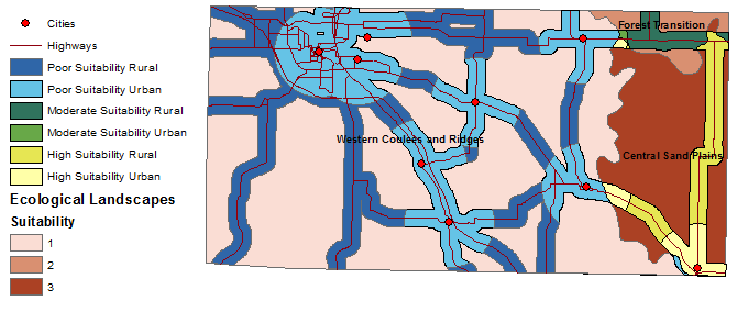Figure 10. Rough map showing areas that make up the six different categories from which addresses will be chosen.

Figure 11. Finished map product with necessary cartographic elements added.

Source Materials 

US Forest Service and cooperators; Ecological Landscapes of Wisconsin (region features); 2003; <ftp://dnrftp01.wi.gov/geodata/ecological_landscapes/>; (12 December, 2014)

Wisconsin Department of Natural Resources; Attitudes Towards Wolves and Wolf Management; August, 2014; <http://dnr.wi.gov/topic/WildlifeHabitat/wolf/documents/WolfAttitudeSurveyReportDRAFT.pdf>; (12 December, 2014)

USDA Economic Research Service; Wisconsin State Fact Sheet; 12 September, 2014; <http://www.ers.usda.gov/data-products/state-fact-sheets/state-data.aspx?StateFIPS=55&StateName=Wisconsin#.VIzkvWOEyRN>; (12 December, 2014)

Wisconsin Department of Natural Resources; Ecological Landscape Associations; 07 October, 2014; <http://dnr.wi.gov/topic/EndangeredResources/Animals.asp?mode=detail&SpecCode=AMAJA01030>; (12 December, 2014)

Lab 4: Vector Analysis With ArcGIS

     Geographic Information Sysytems paired with data from resources such as the DNR can be used to create further useful data and visual graphics. Fortunately the DNR in many states allows public access to data for people to used for adaptation and extracting further data and understandings.

     In Lab 4 our goal was to take data originally accessed from the Michigan Department of Natural resources combine with our ArcGIS suite of programs to generate a cartographic representation of bear habitat in part of Marquette County, Michigan. Along with a map we were tasked with creating a digital data flow model representing the tools and paths used to analyze the given data and adapt features in order to create our map. In the process of this we gained further experience with vector analysis tools including clip, erase, intersect, and dissolve.


Objective I
     The first step for this lab was getting to know our data. This involved checking the file types we were given and what coordinate system the would be represented in in the ArcMap program. 
     We were provided with a file of X,Y coordinates for bear locations within a study area in Marquette county, Michigan. We were also provided with other relevant features of the study area including the study area itself, land cover types, streams, and DNR management areas. The features were originally added to the program as a feature dataset that was not permanent and had limitations as to the tools that could be used. To get around this we simply exported the feature and data, making them a permanent feature class.

Objective II 
     Next we started adding some of the major features including the bear locations, streams and the study areas. By performing a spatial join of the bear coordinate data and the land cover data, we were able to determine what type of cover each of the bears was found in. By summarizing the joined data tables we determined what three habitats the bears were found in most often; mixed forest land, evergreen forest land, and forested wetlands. 
     Knowing that streams are usually an important resource for bears, we calculated the percentage of these bears that were spotted near a stream. To do this we simply selected, by location, bears within 500 meters of a stream and found that 49 of the 68 bears we sighted within this distance of streams. This constituted 72% of the sightings which would lead us to believe it is an important habitat characteristic to bears.

Objective III 
     The data gained in objective two was next used to find possible habitat for bears based on cover types in this study area. To do this we selected the three types where the most bears were found and created a new layer from those selected features. This gave us a new representation of them, but there were still lines that visually separated the types from one another within the single feature. We used the dissolve tool in ArcMap which allowed us to remove all of the lines separating cover types.
     Next, we needed to define the area within 500 meters of all streams as a possible habitat for bears. The original streams feature was expanded using the buffer tool. This tool can create a feature that includes an area of a specified distance around a feature, so we simply chose the streams feature to buffer and specified an area of 500 meters arouund it as the "buffer zone".
     Now we needed to define the area that the bears used for habitat by selecting features that shared both the proximity of 500 meters and the appropriate area of cover. To do this we intersected to two layers created so far in objective three. The intersect tool takes areas of the two features that overlap and turns those sections into another new feature. We now had a feature that displayed areas of bear habitat that had both the right type of cover and the correct proximity to streams while eliminating areas that didn't have both of those properties.

Objective IV 
      For objective four we wanted to find areas of bear habitat that were located within DNR management lands. We simply needed to use the intersect tool again. This would create a new feature showing areas where both the DNR management areas and the proposed bear habitat overlapped. 
     To make things a bit more difficult, the feature showing DNR management areas that we were given was segmented into separate units. We used the dissolve tool again to remove all boundary lines inside of the new feature of DNR managed bear habitat.

Obective V 
      The DNR would likely not want to maintain habitat for bears too close to urban areas as it could bring them in close proximity to people. Therefore we were next assigned to remove any bear management areas within five kilometers of urban or built up areas. 
      To remove management areas within this distance we first defined what areas were urban or built up by selecting them from the land cover feature. We then created a new feature out of that selection just as we did in objective three with the habitat cover types. Next we added a five kilometer buffer like we did for areas near streams in objective three. 
      We now had a feature of an area that could be removed from our map of DNR managed bear habitat. In order to do this we used the erase tool. This tool allows us to select one feature, and then remove areas of another feature that overlap it. We did just this and removed the five kilometer area around urban buildup and erased its features that overlapped the map created in objective four.

Objective VI 
     Finally we were tasked with creating a cartoghraphically pleasing map that showed our proposed bear habitat and areas of it that could be managed by the DNR. This also involved adding a visual reference of the study area within Marquette county and within the state of Michigan. Other necessary elements such as a title, legend, scale bar, and north arrow were then added along with features defining the bear locations and streams in the study area.
(Fig. 1)
     We were also asked to create a data flow model of all of the tools and processes we used to create our map. This can be done using a number of programs that visually aid such a process, but I chose to use the ModelBuilder element of the ArcMap program. This program allows users to select tools from the ArcToolbox directly and drop them into the model being built. It automatically creates representations of the tools that can edited to show input and output representations. 
     Each process can be visually linked in this way to create a model of how the map was developed. The model can also be used in the program to process initial data in the exact manner we did. So if someone were to have data from another county they would simply need to define each variable and this model could run through the process for them. (Fig. 2)

 Results 

Figure 1. Final map including Proposed bear habitat along with areas managed by the Michigan DNR that are within that habitat. Due to their relevance streams and bear locations were also added.

Figure 2. Data flow model used to show what tools (yellow squares) and the input features for those tools (circles). The blue circles represent original sourced features while the green circles represent adapted features created by the tools shown.

 Source Materials 

Michigan Center for Geographic Information; Michigan 1992 NLCD Shapefile by County; 01 November, 2002; <http://www.mcgi.state.mi.us/mgdl/nlcd/metadata/nlcdshp.html>; (04 December, 2014)

Michigan Department of Natural Resources; wildlife_mgmt_units; August, 2001; <http://www.dnr.state.mi.us/spatialdatalibrary/metadata/wildlife_mgmt_units.html>; (04 December, 2014)

Center for Shared Solutions and Technology Partnerships;  Michigan Geographic Framework: Marquette County; 01 June, 2014; <http://www.mcgi.state.mi.us/mgdl/framework/metadata/Marquette.html> (04 December, 2014)